Printed from acutecaretesting.org
January 2010
Verification of methods and instruments
BACKGROUND
Once upon a time routine laboratories had the competence and capacity to develop new principles and methods of measurements; e.g. blood gases by Paul Astrup in Copenhagen, immunological methods for minute hormone concentrations by Leif Wide in Stockholm and Roger Ekins in London.
Also, principles developed in basic science were early explored, e.g. mass spectrometry using isotope dilutions by Ingemar Björkhem in Stockholm in the search for reference methods.
Nowadays, resources of industry are usually required to develop methods for the routine laboratory. However, discovery of new diagnostic markers and techniques to measure their concentration can be traced to a hospital laboratory, e.g. Cystatine C by Anders Grubb in Malmö. In some cases new techniques have led to the establishment of thriving industries, e.g. Hemocue in Ängelholm.
All IVD (in vitro diagnostic devices) instruments and reagents that will be "put on the market" must be documented and approved by an official agency. In Europe the documentation must get a CE mark [1] and in the USA an approval procedure by FDA is mandated.
The approval focuses on risks associated with the use of the devices and documentation of their performance. Much of the responsibility of the IVD performance is hereby transferred from the laboratories to the manufacturers.
The approval procedure requires a thorough validation of the products to show that the device/reagent is fit for purpose. For measurements this includes, but is not limited to, trueness and precision, linearity, chemical interferences, carry-over and risk appraisal. The laboratories must verify that the procedures can be performed at least equally well in-house before they are commissioned to routine investigations.
Laboratories usually limit the verification to compare claims regarding trueness and precision whereas the other criteria may be regarded as inherent to the method/instrument and left to the manufacturer to investigate and bring under control.
Validation and verification are based on statistical procedures. The outcome and interpretation of these depend on the model and what it is designed to illustrate. Thus, the number of samples, repeats, calibrators, sample material and batch-to-batch variation appraisal are input variables that need consideration. Industry and users should agree on these procedures to make the manufacturers' claims and the verification results of the laboratories comparable.
For this purpose international standards and recommendations are available. They may be mandatory but are mostly voluntary, e.g. the ISO standards. Standards rarely give concrete instructions or worked examples. However, guidance documents or recommendations provide exactly that.
Recommendations and standards will not be widely accepted and applied unless they capture the users' different needs and expectations. Although electronic communications have simplified and shortened the consensus procedure, it may still take several years for a document to become accepted.
Besides ISO and CEN, IFCC (International Federation of Clinical Chemistry and Laboratory Medicine), JCTLM (Joint Committee for Traceability in Laboratory Medicine, an international consortium sponsored by the Bureau International des Poids et Mesures) and CLSI (Clinical and Laboratory Standards Institute) produce standards and recommendations.
Briefly, the IFCC represents national professional societies, the JCTLM has several stakeholders from the profession, industry and metrology. CLSI is a non-profit organization that coordinates volunteer contributions from representatives of the profession, the regulatory agencies and industry.
The CLSI has published a series of documents on the evaluation of laboratory methods, i.e. the Evaluation Protocols (EP). Recently, the ACB (Association for Clinical Biochemistry) in the UK published free downloadable documents and software [2] which describe minimal, yet powerful verification procedures in the laboratory.
IMPRECISION FROM PATIENT SAMPLES OR REFERENCE MATERIALS
Imprecision is the numerical expression of precision and is reported as the standard deviation or coefficient of variation. The standard deviation is the square root of the variance and the coefficient is the standard deviation relative to the mean of the measurements.
When the standard deviation is calculated from repeated measurements of the same sample and unchanged conditions, the repeatability or within-series variation is obtained. The mean of the standard deviation is underestimated, for mathematical reasons, if only few observations are considered; e.g. if based on two observations, the mean underestimate is about 20 % with a considerable dispersion.
Therefore, it is imperative that any estimation of the standard deviation is based on a sufficient number of observations (Fig. 1).
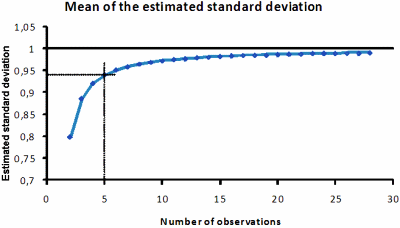
FIG. 1. The mean of the standard deviation estimated from an increasing number of observations. In the simulation the standard deviation was set to 1, which is practically achieved with 20-25 observations.
If conditions change between estimating the imprecision, e.g. from one day to another or after recalibration of the measurement procedure, the imprecision is characterized as between-series imprecision. The end user is more interested in the combined imprecision or the intra-laboratory imprecision which can be estimated from the repeatability and the between-series imprecision. The laboratory needs to establish efficient methods to estimate all three types of imprecision.
The between-run variation is best estimated using a statistical procedure, the ANOVA, i.e. analysis of variation. The ANOVA may be best known from estimating if there is a statistical difference between several series of measurements and its results are presented to answer that question in a standardized manner in most statistical packages and spreadsheet programs. The standard output is shown in Table I.
| Source of Variation |
SS |
df |
MS |
F |
| Between Groups Within Groups Total |
74.8 |
4 |
18.7 |
28.3 |
An ANOVA can also be used to estimate the within- and between-series variation and provides a method to estimate the within-laboratory variation. The MSw is the mean sum of square and is equal to the within-series variance. The MSb includes the within-series variation and needs to be compensated:
![]() [1]
[1]
where n is the mean number of observations in the series. The is the "purified between-series variance", also called the "unbiased between-series variance" in statistical literature. The total, combined or intra-laboratory variance is
+MSw [2]
If the above correction is not made and the within-laboratory variance were estimated as the sum of MSb and MSw, it would be grossly overestimated.
At least five observations during five runs are suggested in the ACB software but up to 10 observations in up to 10 series can be accommodated in the program; the more observations the more reliable the results will be. The program will make all the calculations and display the outcome in a table and graph (Fig. 2, Table II).
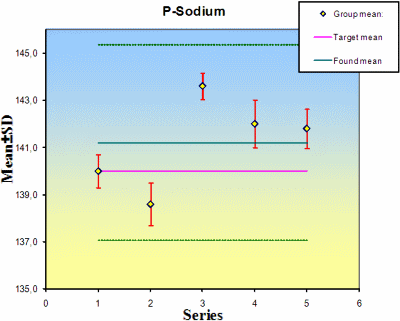
FIG. 2. The mean and standard deviations of the series or runs in an estimation of the precision. If a value of the used material is known, this is shown (solid violet line). The mean and standard deviations of the observations are shown in green.
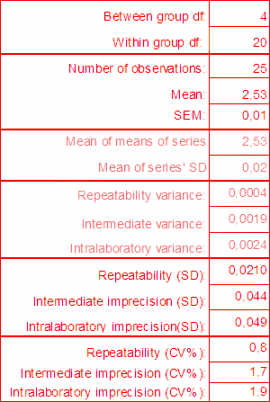
If in measurements the MSb were smaller than the MSw, a negative Sb2 [1] would result. By convention the MSb is then set to zero and the intra-laboratory variance is equal to the within-series variance.
An estimate of the intra-laboratory variation can either be made as a particular study according to the ACB protocol or by using data collected during weeks. Routinely obtained IQC data accumulated during a month with 2-3 daily replicate measurements can be used.
There will be 30 series in the ANOVA, each with 2-3 observations. In spite of the few within-day observations, the within-series degrees of freedom will be large and the estimates quite reliable. The program is not designed for this design but the calculations can easily be performed in a spreadsheet using the ANAOVA function and the formulas above for the calculation of the between-series variance [1] and intra-laboratory variation [2].
If the variance were estimated from all observations as if they belonged to one homogeneous dataset, this would lead to an underestimate of the intra-laboratory variance because the between-series variation is not taken into account. The magnitude of the underestimate cannot be stated in general terms. If such a value is used to establish IQC limits, the risk of "false alarms" will increase, which may affect the cost of quality management and increase the turnaround time.
The ANOVA approach can also be used to establish the total variation with several instruments involved. It will then be important to use more than five observations in each series to ascertain a reasonable within-series variance.
These procedures can be carried out with patient material, provided there is enough for the entire series, but equally well with reference materials. The advantage of using material with a known concentration is that the bias can be estimated in the same procedure.
ESTIMATION OF BIAS FROM PATIENT MATERIAL
Traditionally, laboratories compare a new measurement procedure with previous ones by splitting samples into aliquots that are measured by the new (test) and a comparative method as close in time as possible. This procedure has been described in both the CLSI EP9 and EP15. The ACB provides a flexible program that easily handles this situation.
The program allows single or duplicate measurements and estimates a number of statistics that will assist the laboratory to evaluate the performance. There are not too many reference methods available and this approach will therefore not address the bias as defined metrologically but rather the difference between the selected methods.
It is important that the chosen samples are representative and that they cover the entire measuring interval. Outliers in the central part of the measuring interval tend to have little impact on the regression whereas outliers at the ends of the interval may have a large impact. Any outlier will have an effect on the correlation coefficient (r).
In the following, functions will be discussed that are included in the ACB software and the figures are copied from those spreadsheets. There is much more information available than the regression and bias if samples have been properly selected and carefully measured.
Therefore, the philosophy of the software is to allow as much flexibility as possible and leave it to the user to pick and choose and evaluate the results guided by some instructions. The software allows the input of up to 100 samples, as single measurements or duplicates.
Before the statistical evaluation is performed, the scatterplot (Fig. 3) and difference plots should be carefully studied to identify outliers that may be candidates for deletion, and at least they indicate possible problems with the measuring system. To assist this procedure the difference between individual measurements are shown and the maximal flagged.
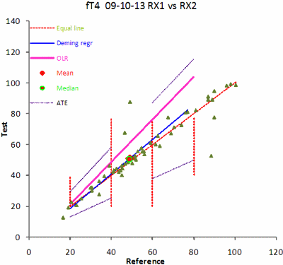
FIG. 3. The scatterplot. Vertical red lines are the limits of the partitions that can be changed by the operator. The mean and the median of the selected dataset are shown. The graph displays the equal line (dotted), the Deming regression (blue), the OLR regression (violet) and the ATE lines (dotted purple), in this case for the low and high partitions.
Basic statistics are calculated for the datasets, e.g. mean, standard deviation, to characterize the sample population.
The significance of the difference between the methods is evaluated by the Student's t-test of dependent variables tdep. This test requires that the differences are normal distributed. The dataset and the distribution of the dataset can therefore be truncated, which is described in more detail below.
The data are used for various more advanced calculations, e.g. the regression function, i.e. the slope and intercept and the correlation coefficient. The ordinary regression (OLR) requires that the analytical variance of the dependent variable (Y) is much larger than that of the independent variable (X). If that is not the case, a better regression would be an orthogonal regression and the choice is the Deming regression.
Both options are available and either can be displayed in the scattergram. However, the Deming regression requires that the variance of the method is defined. The ACB program allows input of results as singles or duplicates. If duplicates have been entered, then the analytical imprecision of the methods is calculated and will be input to the Deming regression.
In any case the operator can define the analytical imprecision of the dependent and independent variables and enter them independently – it may be that the imprecision of the methods has been carefully established in separate experiments. As the analytical variance of the dependent variable increases relative to that of the independent one, the Deming regression function approaches that of the OLR.
The Passing-Bablok regression has the advantage of being less sensitive to outliers and has no requirements to the distribution of the data. The calculation of the Passing-Bablok requires a special program.
The regression function may differ in different parts of the measuring interval which means that the datasets are not linearly correlated. It is therefore valuable to consider partitioning the dataset, and the program allows up to three partitions. The average bias and the Student's tdep are then displayed for each partition. The partitioning also allows truncating the dataset at the high or low concentrations or both.
If truncated, the new dataset will be used as the basis for the bias calculation. To be meaningful the number of observations needs to be large enough to allow about 20 observations in each partition.
The differences between the means of each of the observations and their means are presented and the maximum differences are flagged. The operator can toggle between the differences of the means or either of the results of the test or comparative methods.
This facilitates the identification of potential outliers. The differences are also graphically displayed (Fig. 4) in difference graphs. These are traditional Bland-Altman graphs but the program also allows the differences to be displayed versus the results of the comparative method. This is usually recommended if the comparative method is a reference method. The two diagrams show the absolute and relative differences between results, and the trend of the differences.
The confidence limits of the differences are calculated but should be considered with caution. The estimated confidence level is only truly valid if the distribution of the differences is normal or close to normal. As mentioned above this is also a prerequisite for applying the Student's tdep test.
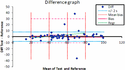
FIG. 4. The difference graph. The mean of all observations and their trend line, the mean ±2 s of the selected differences and the limits of the selected subsample (dot-dash line) after truncation of the differences are shown.
A deviation from normality often leads to long tails and it thus becomes necessary to present some indication of normality. The skewness (peakedness) of the distribution of the differences is displayed as it is one of the characteristics of a normal distribution. If the skewness is within –1 < skewness < 1, the skewness is generally regarded as being minor.
If not, the distribution of the differences can be truncated and thus improve the validity of the calculations. The total number of observations left after a truncation should be considered.
Thus, there are several means to adjust the dataset. Obvious outliers, identified from the graphs or the tables of differences, can simply be deleted from the input table. The dataset itself can be truncated, which is particularly convenient if there are samples with very high or very low concentrations.
Finally the distribution of the differences can be truncated. The dataset that is eventually included in the evaluation is the smallest that is obtained after truncation of both the dataset and the differences.
The clinical performance of a procedure, often used in risk assessment, can be described as the number of observations that fall outside a certain deviation from the equal line or regression line, ATE (Allowable Total Error). The remaining are outside the Limit of Erroneous Results (LER). In the program the ATE can be set for the low, mid or high concentration limits and optionally displayed in the scattergram.
The program will calculate the number of results in the ATE and LER sectors of the comparison. This may be different depending on if the ATE and LER are estimated in relation to any of the regressions or the equal line.
CONCLUSION
A standardized procedure for laboratory verification of precision and trueness is described in terms of a non-proprietary and downloadable software package.
References1. EU IVD directive 98/79 http://eur-lex.europa.eu/LexUriServ/LexUriServ.do?uri=CELEX:31998L0079:EN:NOT
References1. EU IVD directive 98/79 http://eur-lex.europa.eu/LexUriServ/LexUriServ.do?uri=CELEX:31998L0079:EN:NOT
May contain information that is not supported by performance and intended use claims of Radiometer's products. See also Legal info.
Acute care testing handbook
Get the acute care testing handbook
Your practical guide to critical parameters in acute care testing.
Download nowScientific webinars
Check out the list of webinars
Radiometer and acutecaretesting.org present free educational webinars on topics surrounding acute care testing presented by international experts.
Go to webinars


